1. 项目介绍
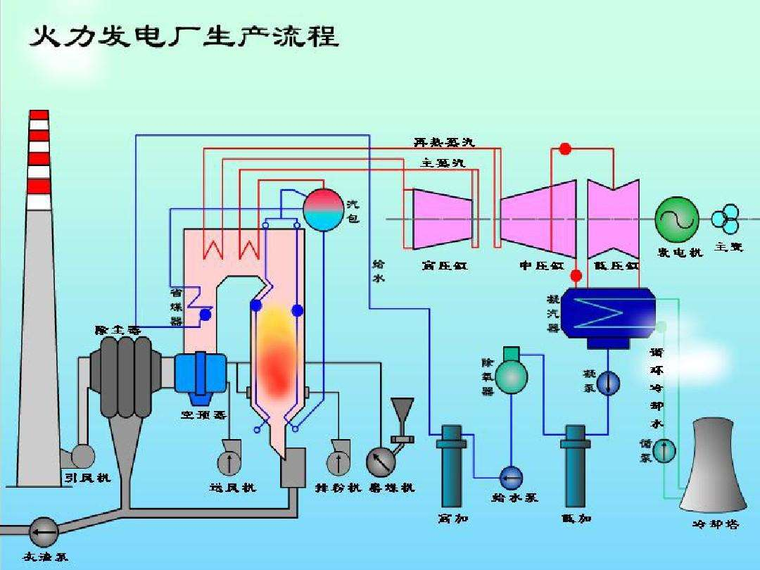
火力发电的基本原理是:燃料在燃烧时加热水生成蒸汽,蒸汽压力推动汽轮机旋转,然后汽轮机带动发电机旋转,产生电能。在这一系列的能量转化中,影响发电效率的核心是锅炉的燃烧效率,即燃料燃烧加热水产生高温高压蒸汽。
锅炉的燃烧效率的影响因素很多,包括:
- 锅炉的可调参数:如燃烧给量,一二次风,引风,返料风,给水水量
- 锅炉的工况:如锅炉床温、床压,炉膛温度、压力,过热器的温度等
本项目将探索这些因素与发电效率的关系,通过数据分析找出关键影响因素。
2. 数据准备与概览
首先导入必要的数据分析库:
import numpy as np
import pandas as pd
import matplotlib.pyplot as plt
import seaborn as sns
from scipy import stats
import warnings
warnings.filterwarnings("ignore")
加载训练集和测试集数据:
train_data_file = "./data/zhengqi_train.txt"
test_data_file = "./data/zhengqi_test.txt"

train_data = pd.read_csv(train_data_file, sep='\t')
test_data = pd.read_csv(test_data_file, sep='\t')
查看训练数据基本信息:
train_data.info()
test_data.info()
train_data.describe(include='all')
train_data.head()
3. 数据可视化分析
3.1 箱线图分析
箱线图可以帮助我们直观地观察数据分布、识别异常值:
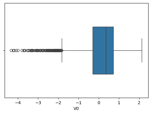
创建所有特征的箱线图:
column = train_data.columns.tolist()[:39]
fig = plt.figure(figsize=(20, 40))
for i in range(39):
    plt.subplot(13, 3, i + 1)
    sns.boxplot(train_data[column[i]], orient="v", width=0.5)
    plt.ylabel(column[i], fontsize=8)
3.2 特征分布比较
使用核密度估计图比较训练集和测试集的特征分布:
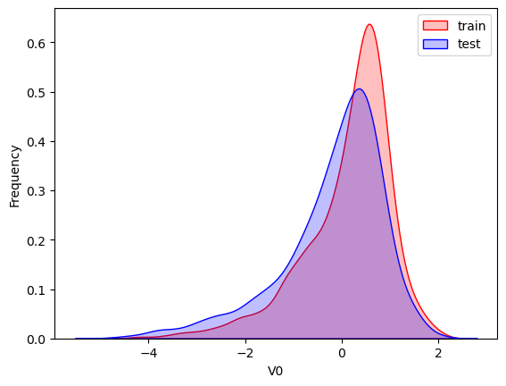
# 绘制所有特征的分布对比
dist_cols = 6
dist_rows = len(test_data.columns)
plt.figure(figsize=(4 * dist_cols, 4 * dist_rows))

i = 1
for col in test_data.columns:
    ax = plt.subplot(dist_rows, dist_cols, i)
    ax = sns.kdeplot(train_data[col], color="Red", shade=True)
    ax = sns.kdeplot(test_data[col], color="Blue", shade=True)
    ax.set_xlabel(col)
    ax.set_ylabel("Frequency")
    ax = ax.legend(["train", "test"])
    i += 1
3.3 特定特征分析
分析特征’V5’, ‘V17’, ‘V28’, ‘V22’, ‘V11’, ‘V9’的分布:
col = 3
row = 2
plt.figure(figsize=(5*col, 5*row))
i = 1
for c in ["V5", "V9", "V11", "V17", "V22", "V28"]:
    ax = plt.subplot(row, col, i)
    ax = sns.kdeplot(train_data[c], color="Red", shade=True)
    ax = sns.kdeplot(test_data[c], color="Blue", shade=True)
    ax.set_xlabel(c)
    ax.set_ylabel("Frequency")
    ax = ax.legend(["train", "test"])
    i += 1
4. 相关性分析
4.1 特征相关性热力图
根据观察到的分布情况,筛选掉部分特征后分析相关性:
drop_col_kde = ["V5", "V9", "V11", "V17", "V22", "V28"]
train_data_drop = train_data.drop(drop_col_kde, axis=1)
train_corr = train_data_drop.corr()
绘制相关性热力图:
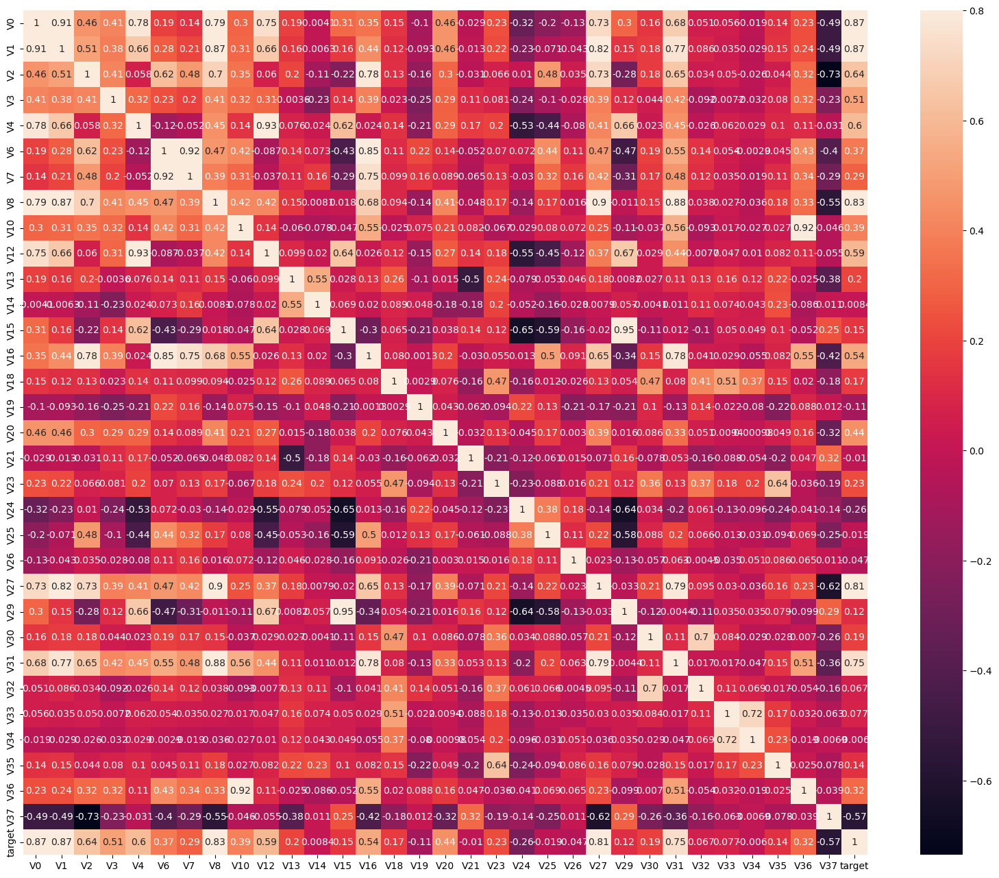
4.2 半热力图
plt.figure(figsize=(24, 20))
mcorr = train_data_drop.corr()
mask = np.zeros_like(mcorr, dtype=np.bool_)
mask[np.triu_indices_from(mask)] = True
cmap = sns.diverging_palette(220, 10, as_cmap=True)
g = sns.heatmap(mcorr, mask=mask, cmap=cmap, square=True, annot=True, fmt="0.2f")
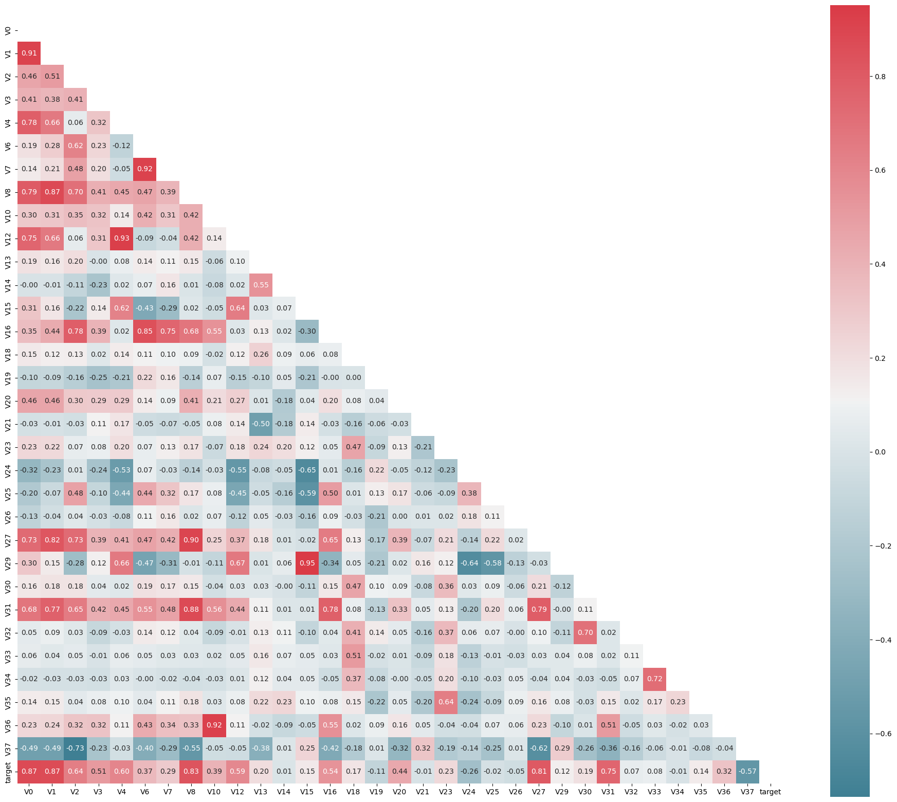
5. 特征筛选
根据与目标变量的相关性进行特征筛选:
cond = mcorr['target'].abs() < 0.1
drop_col_corr = mcorr.index[cond]
train_data.drop(drop_col_corr, axis=1, inplace=True)
test_data.drop(drop_col_corr, axis=1, inplace=True)
6. 数据预处理
合并训练集和测试集,添加标签并保存:
train_data["label"] = "train"
test_data["label"] = "test"
all_data = pd.concat([train_data, test_data])
all_data.to_csv('./processed_zhengqi_data.csv', index=False)
7. 结论
通过探索性数据分析,我们:
- 识别了训练集和测试集中分布不一致的特征
- 分析了各特征与目标变量的相关性
- 筛选出相关性较低的特征并移除
- 为后续建模做好了数据准备工作
下一步我们将基于这些处理过的数据进行模型构建和评估。